ussie
ussie.Rmd
library(ussie)
library(dplyr)
#>
#> Attaching package: 'dplyr'
#> The following objects are masked from 'package:stats':
#>
#>     filter, lag
#> The following objects are masked from 'package:base':
#>
#>     intersect, setdiff, setequal, union
ussie helps standardize European football data tables retrieved from the engsoccer package for each country.
spain <- uss_make_matches(engsoccerdata::spain, "Spain")
glimpse(spain)
#> Rows: 23,915
#> Columns: 8
#> $ country       <chr> "Spain", "Spain", "Spain", "Spain", "Spain", "Spain", "S…
#> $ tier          <fct> 1, 1, 1, 1, 1, 1, 1, 1, 1, 1, 1, 1, 1, 1, 1, 1, 1, 1, 1,…
#> $ season        <int> 1928, 1928, 1928, 1928, 1928, 1928, 1928, 1928, 1928, 19…
#> $ date          <date> 1929-02-10, 1929-02-10, 1929-02-10, 1929-02-10, 1929-02…
#> $ home          <chr> "Arenas de Getxo", "Espanyol Barcelona", "Real Madrid", …
#> $ visitor       <chr> "Atletico Madrid", "Real Union", "CE Europa", "Athletic …
#> $ goals_home    <int> 2, 3, 5, 1, 0, 1, 9, 0, 3, 5, 3, 3, 1, 0, 2, 1, 2, 3, 2,…
#> $ goals_visitor <int> 3, 2, 0, 1, 2, 2, 0, 3, 1, 2, 0, 1, 1, 4, 1, 2, 1, 0, 2,…
Get data from a specific country
uss_get_matches() can retrieve data for a specific country (among those available) within the engsoccer dataset
spain_matches <- uss_get_matches("spain") |> glimpse()
#> Rows: 23,915
#> Columns: 8
#> $ country       <chr> "Spain", "Spain", "Spain", "Spain", "Spain", "Spain", "S…
#> $ tier          <fct> 1, 1, 1, 1, 1, 1, 1, 1, 1, 1, 1, 1, 1, 1, 1, 1, 1, 1, 1,…
#> $ season        <int> 1928, 1928, 1928, 1928, 1928, 1928, 1928, 1928, 1928, 19…
#> $ date          <date> 1929-02-10, 1929-02-10, 1929-02-10, 1929-02-10, 1929-02…
#> $ home          <chr> "Arenas de Getxo", "Espanyol Barcelona", "Real Madrid", …
#> $ visitor       <chr> "Atletico Madrid", "Real Union", "CE Europa", "Athletic …
#> $ goals_home    <int> 2, 3, 5, 1, 0, 1, 9, 0, 3, 5, 3, 3, 1, 0, 2, 1, 2, 3, 2,…
#> $ goals_visitor <int> 3, 2, 0, 1, 2, 2, 0, 3, 1, 2, 0, 1, 1, 4, 1, 2, 1, 0, 2,…
We can add filtering conditions as well:
spain_1987_matches <- uss_get_matches("spain", season == 1987,
                                      home == "Real Madrid" | visitor == "Real Madrid") |>
    uss_make_teams_matches()
We can also accumulate seasons:
spain_1987_matches |>
  uss_make_seasons_cumulative() |>
  dplyr::arrange(team, date)
#> # A tibble: 76 × 12
#> # Groups:   country, tier, season, team [20]
#>    country tier  season team        date       matches  wins draws losses points
#>    <chr>   <fct>  <int> <chr>       <date>       <int> <int> <int>  <int>  <int>
#>  1 Spain   1       1987 Athletic B… 1987-10-31       1     0     1      0      1
#>  2 Spain   1       1987 Athletic B… 1988-03-12       2     0     1      1      1
#>  3 Spain   1       1987 Atletico M… 1987-11-07       1     1     0      0      2
#>  4 Spain   1       1987 Atletico M… 1988-03-20       2     1     0      1      2
#>  5 Spain   1       1987 CA Osasuna  1987-09-20       1     0     0      1      0
#>  6 Spain   1       1987 CA Osasuna  1988-02-13       2     1     0      1      2
#>  7 Spain   1       1987 Cadiz CF    1987-08-30       1     0     0      1      0
#>  8 Spain   1       1987 Cadiz CF    1988-01-31       2     0     0      2      0
#>  9 Spain   1       1987 CD Logrones 1987-12-06       1     0     0      1      0
#> 10 Spain   1       1987 CD Logrones 1988-04-10       2     0     0      2      0
#> # … with 66 more rows, and 2 more variables: goals_for <int>,
#> #   goals_against <int>
#> # ℹ Use `print(n = ...)` to see more rows, and `colnames()` to see all variable names
Plot results over seasons
Of the countries included in uss_countries(), only "england" has data for more than one tier, where we can see the effects of relegation and promotion. You can use uss_plot_seasons_tiers() to look at performance over seasons, using data returned from uss_make_seasons_final():
leeds_norwich <-
  uss_get_matches("england") |>
  uss_make_teams_matches() |>
  filter(team %in% c("Leeds United", "Norwich City")) |>
  uss_make_seasons_final() |>
  arrange(team, season)
leeds_norwich
#> # A tibble: 178 × 12
#> # Groups:   country, season, tier [155]
#>    country tier  season team        date       matches  wins draws losses points
#>    <chr>   <fct>  <int> <chr>       <date>       <int> <int> <int>  <int>  <int>
#>  1 England 2       1920 Leeds Unit… 1921-05-07      42    14    10     18     38
#>  2 England 2       1921 Leeds Unit… 1922-05-06      42    16    13     13     45
#>  3 England 2       1922 Leeds Unit… 1923-05-05      42    18    11     13     47
#>  4 England 2       1923 Leeds Unit… 1924-05-03      42    21    12      9     54
#>  5 England 1       1924 Leeds Unit… 1925-05-02      42    11    12     19     34
#>  6 England 1       1925 Leeds Unit… 1926-05-01      42    14     8     20     36
#>  7 England 1       1926 Leeds Unit… 1927-05-07      42    11     8     23     30
#>  8 England 2       1927 Leeds Unit… 1928-05-05      42    25     7     10     57
#>  9 England 1       1928 Leeds Unit… 1929-05-04      42    16     9     17     41
#> 10 England 1       1929 Leeds Unit… 1930-05-03      42    20     6     16     46
#> # … with 168 more rows, and 2 more variables: goals_for <int>,
#> #   goals_against <int>
#> # ℹ Use `print(n = ...)` to see more rows, and `colnames()` to see all variable names
The default is to show the wins on the y-axis:
uss_plot_seasons_tiers(leeds_norwich)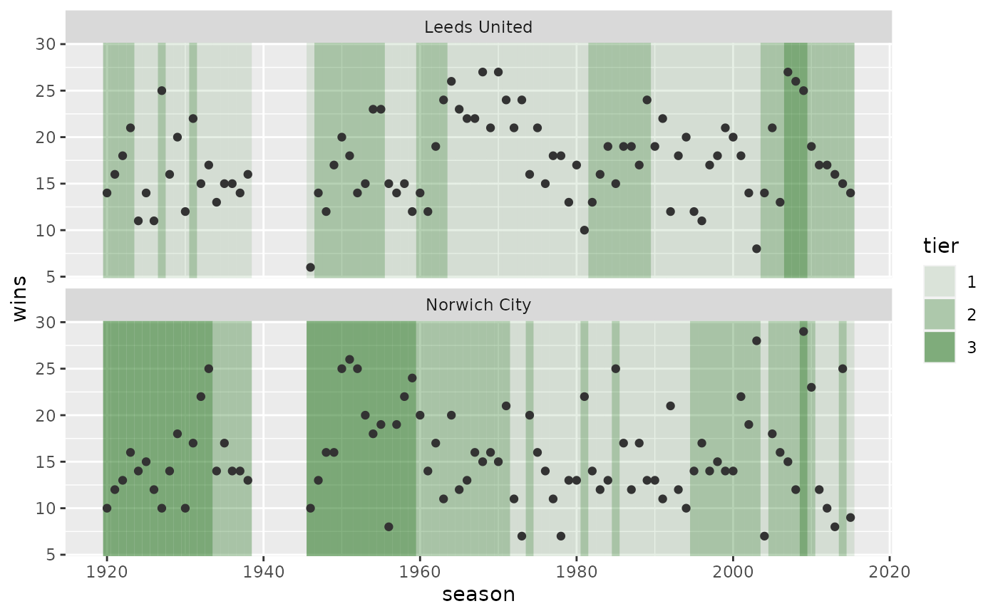
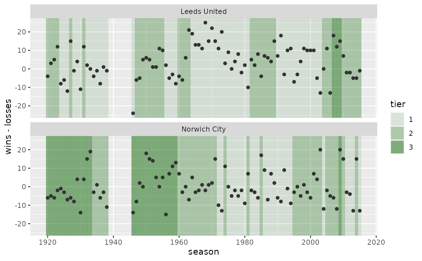
You can provide an argument, aes_y, where you can supply an expression just as you would for ggplot2:
uss_plot_seasons_tiers(leeds_norwich, aes_y = wins - losses)